Image Injection Detection
IP Available
Code Reference implementation for Android implemented in Java, Kotlin and Renderscript.
Patent Title: COMPUTER VISION BASED APPROACH TO IMAGE INJECTION DETECTION
Pub . No: US 2021/0295075 A1
Pub . Date: Sep. 23, 2021
Status: pending
Introduction
One possible method to circumvent a verified-capture solution is though image injection.
In this scenario, a malicious user injects/overlays a desired image into the mobile device’s visual input stream. We propose this can be negated through a computer- vision based approach.
Preliminaries
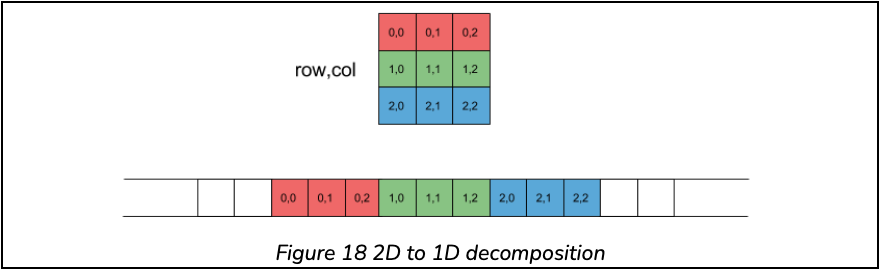
Although novel methods were proposed and evaluated, many of them were computationally expensive for a mobile device. Such as pixel velocity tracking – which provided a favourable matching accuracy but remained costly. Therefore we have turned to 1-d correlation algorithms, which are dependent on raw pixel data from a given set of images. Notably, the two-dimensional data, that is an image, was reduced to a single dimension as illustrated in Figure 18.
Reducing the dimension of the data allows for spoof detection on Android devices, while maintaining a low computational cost. Moving Forward from this, the second need was the ability to identify an Image, whilst removing spatial information related to an Image. Meaning that this work complies with Serelay’s logic, that a given image could never be passed through to its backend for post processing, and rather its metadata, or any non-reconstructive data for that matter, is allowed.
With this in mind, this work draws back the idea of Image Classification through the introduction of image distributions, developed in the late 70s. Tan- gent to this research, work related to image feature detection showed promising results in conjunction, but was limited by its computational complexity – and hence the exploration of this method.
We create a unique fingerprint of a capture sequence under an associated colour space. With these fingerprints a correlation-based approach, or methods alike, are adapted to classify the image as (1) Matched or (0) Spoofed.
Colour spaces
RGB is the predominant colour space used in many electronic devices, as opposed to others like HSL or HSV. However, since we are dependent on raw pixel information, RGB tends to distort its classification model. For example, take the red colour space seen in Figure 19.
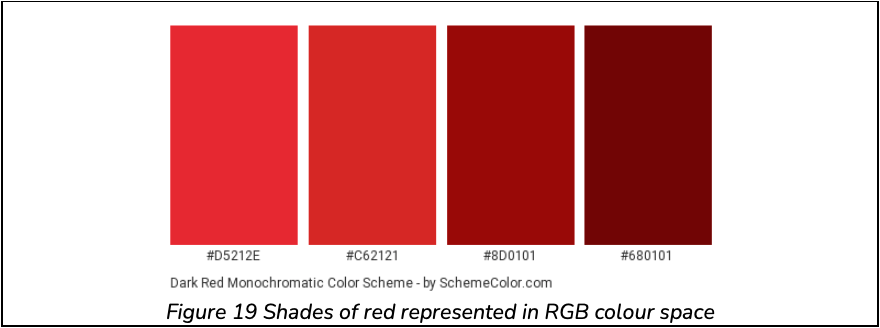
Under inspection of these, we may want to classify these colours as spoofed. But what we fail to understand is that this is red under different light intensities (through RGB colour mixing). With this in mind, in a realisable scenario, a camera feed is introduced to an enormous amount of noise. For example, planar, depth and light variation are one of few noise samples in this classification problem. Notably, light variation is the most predominant factor. Depth on the other hand, is to somewhat dependent on light, and is filtered simultaneously.
This work seeks to remove light distortion, in order to mitigate a potential high false positive rate, by moving from RGB’s to HSV’s colour space.
HSV, Hue Saturation Value, is a Cylindrical Colour space. Such that a RGB pixel of ([0 → 255], [0 → 255], [0 → 255]) is transformed to an angle ([0 → 360]) in the hue space. Its relationship
-
Red: 0◦→ 60◦Hue.
-
Green: 121◦→ 180◦Hue.
-
Blue 241◦→ 300◦Hue.
Saturation, on the other hand, describes the amount of grey in a particular colour, from 0 to 100 percent. This type of information is valuable in identifying images taken by different cameras, or under different internal parameters setting (assuming no post editing has been performed). Which may be used as a factor in classifying a spoofed image.
Lastly, Value works in conjunction with saturation and describes the brightness or intensity of the colour, from 0-100%, where 0% is dark, while a 100% is the brightest and reveals the most colour. In other words, this captures light information about a given scene.
As mentioned, this work aim is to remove the light noise that are physically realisable. And for this reason, V (Valued) has been dropped in its classification algorithm.
Colour Distribution
Using HS (Hue and Saturation) a statistical distribution model, or in simpler terms a histogram plot of colour pattern, is obtained for each image. But given the continuity of the HSV space, and the device constraints, a Nearest Neighbour approach was applied to the HS image data. At the time of work, the NN algorithm was constrained to 1◦and 1% for Hue and Saturation respectively.
The distribution, hist HS of dimension [1×460], data was then L2 normalised. Its transformation is as follows,
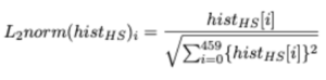
A second thing to note, that by creating a colour distribution all spatial-visual information about an image is dropped and reconstruction is not possible.
A third point is that histograms are invariant to translation and they change slowly under different view angles, scales and in presence of occlusions.
A final remark is that there is a potential threat to spoof a histogram. However, to do this in real time it be would require knowing the distribution of the camera feed (the current scene) and process the intended injected image simultaneously. However, this is not plausible.
Matching
For a given set of images, we can now construct a distribution function related to each image. These functions are assumed to be independent, mutually exclusive and random from each other, and hold a strong positive correlation when two fingerprints are alike, i.e., the same image is matched. With this in mind, matching between such function is per- formed under a correlation-based approach. This work explores and formulates various correlation-based methods. As a note, correlation in this work deviates from its traditional definition – and for this reason is can be considered a distance measure function, because some methods explored are not normalised between 0 → 1 as expected. This loose definition is taken advantage of in device testing.
The correlation methods explored in this paper are as follows:
-
Zero-Normalised Cross-Correlation (Variant)
-
Chi-squared statistic
-
Intersection
-
Bhattacharyya distance
Zero Normalised Cross Correlation
Zero Normalised Cross-Correlation (ZNCC) is the most used method in the field of digital signal processing. And an interesting fact is that it is inherently embedded in Kernel Functions for SVM classifiers. But basically, it is a similarity measure of two distribution functions that are relatively dis- placed from each other. This means that ZNCC is a shift invariant kernel, which offers benefits to situation with various lighting. So instead of using colour data a hard fact, we consider its shape. This is best explained by an illustration.
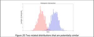
From Figure 20, notice that the two distribution functions, blue and red, tend to peak and trough in a similar pattern. This illustration is an attempt to simulate a scenario when there is uncontrollable variation to global lighting. Notably, even though we are considering an HS distribution there is a potential gap for disturbances and hence this needs to be accounted for. The outcome of this scenario would produce two distribution functions of the same shape, but different intensities. ZNCC aids in tackling this problem.
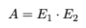
A variant of ZNCC is introduced by this work to match two distribution functions, E1(i) and E2(i) respectively. It is formally defined by,
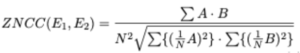
Where:
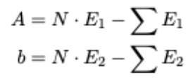
The correlation metric is, ZNCC(E1,E2)∈[0,1]. And following relationship:
![]()
Chi-Squared statistic
This work draws on the field of statistics and manipulates it to fit the task at hand. Traditionally the Chi-Squared statistic is a test that measures how expectations compare to actual observed data. With its purpose in mind, the data within this work is assumed to be observed. Now given two distributions, E1 and E2, we assume that E1 is the observed expectation; this is allowed by making a second assumption that E1 and E2 are random, raw, mutually exclusive, drawn from independent variables and from a large enough sample space.
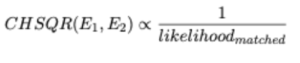
Formally the matched likelihood is determined by
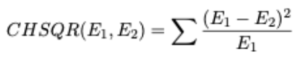
Where CHSQR(E1, E2) ∈ R, and
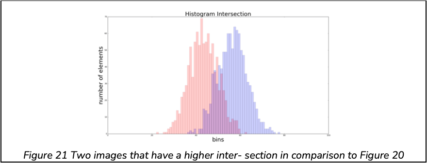
Intersection
The Intersection correlation based method makes use of a non-linear feature mapping function, min(a, b). As the name suggests, it determines the intersection between two distributions functions. For example, in Figure 20, the intersection between the histograms is small as opposed to Figure 21.
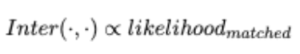
Mathematically, the similarity between two frames (E1, E2) is determined by,
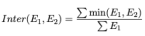
So Inter(E1, E2) ∈ R, and
Bhattacharyya distance
The Bhattacharyya coefficient is a normalised measure of separability, or in other words it is a measurement of the amount of overlap between two statistical samples. Here we use Bhattacharyya as a distance measure between two observed functions, E1, E2. With a variant of the form,
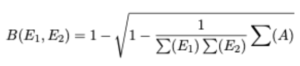
Where
So B(E1, E2) ∈ R, and
Dataset overview
Since the main focus of this work is to classify between (1) Matched, or (0) Spoofed – the two datasets were obtained to simulate these scenarios for hypothesis testing.
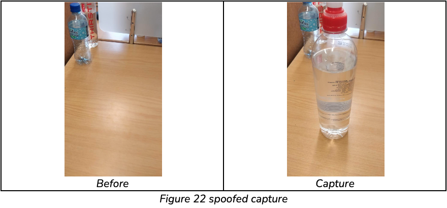
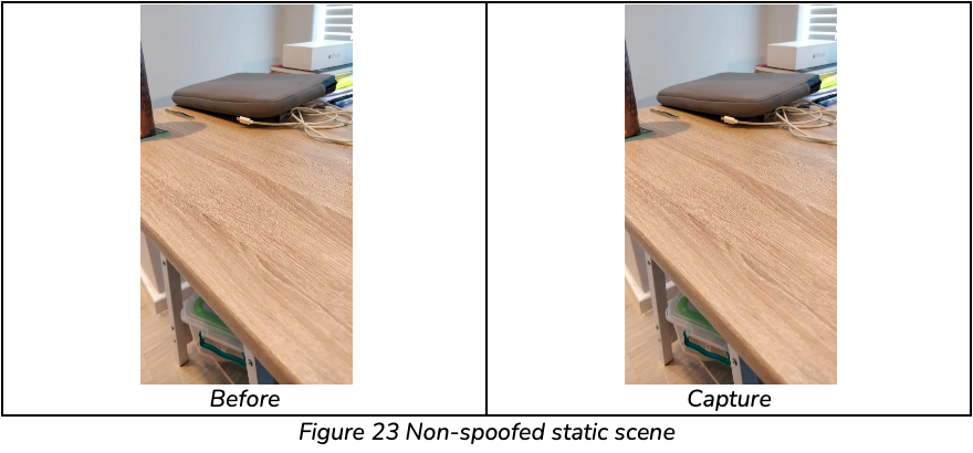
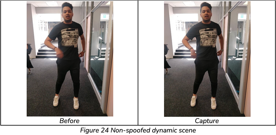
Specifically, a single set consisted of a sequence of preview frames before, and after, capture and a single capture frame. For hypothesis Testing, 4 preview frames were gathered before and after capture. This provided a good basis to evaluate the correlation methods, and the distribution approach combined, over a single sequence. The second set of testing was done on a mobile device. This allowed for a more realistic set to be collected. Except here, the set only observed 1 preview frame before, and after, capture and a single capture frame. Spoofed and non-spoofed examples can be observed in Figure 22, Figure 23, and Figure 24.
Additionally, the initial dataset, that was used to determine final cost function, was composed of 167 sample points.
Hypothesis testing
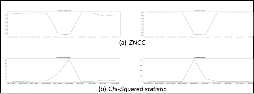
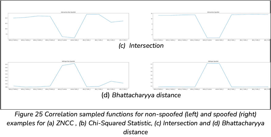
The four correlation methods were tested across the spoofed and non-spoofed dataset. Their respected results are seen in Figure 25.
From Figure 25, the first thing to note is the sudden difference in correlation moving from the 4th before preview to capture and again from capture to the 1st after preview, regardless of spoofed or non-spoofed. This is because the captured image requires a longer processing time, under different exposures, shutter speeds and white balance. This passed time inherently allows the scene to change and hence attributes the offset correlation encoded. Notably, these parameters change per scene, and therefore the timing difference between previews and captures change accordingly.
From Figure 25 we take note of the sensitivity of Chi-Squared to spoofed images. This is seen as a valued 14 moves to 8000 for a non-spoofed and spoofed set respectively on preview-before-4 to capture. In addition, Bhattacharyya, Intersection and ZNCC are able to distinguish between spoofed and non-spoofed, with a sensitivity tending towards non-spoofed images.
Device implementation
All correlation algorithms were tested in python using the supported CV libraries. Moving towards implementation on Android, this work wished to act as a set of standalone functions.
To determine the distribution function for a set of images, as mentioned before, we require that the images (in RGB) be converted to an HS histogram. This is computationally expensive, especially with a growing Bitmap resolution. For a single image it requires X × Y iterations. Where X and Y are the image’s dimensions. For this reason, RenderScripts were used to convert the images, and obtain their respective distributions. RenderScripts are a frame- work for running computationally intensive tasks at high performance on Android – utilising multi-core CPUs and GPUs.
The correlation calculations were implemented from first principles using their associated derivations presented in earlier.
Device testing
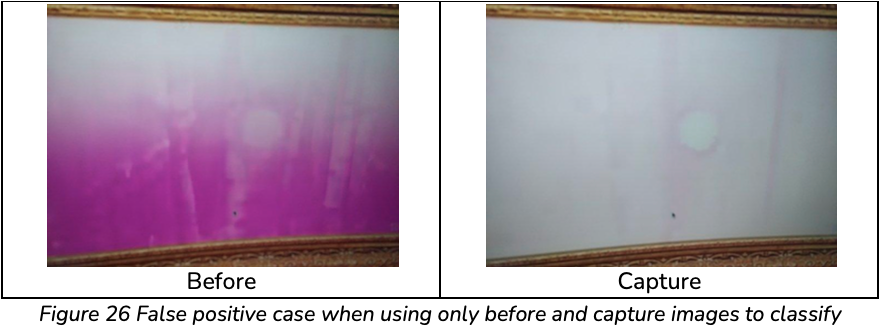
Initially, a single preview before and on capture was utilised to classify between spoofed and non- spoofed. However, it was found that in different scenarios it fails. For example, in Figure 26, we observe a scene with flashing images in which the correlation methods classify as spoofed. This was mitigated by including a preview after capture.
Cost Function
After sensitivity analysis, it was found that CHSQR was far more sensitive to spoofed images in comparison to Bhattacharyya and Intersection. While Bhattacharyya and Intersection were sensitive to non-spoofed images. Given this the following cost function was derived and implemented.

With this a threshold of 0.1 was defined. This gives a classification function δ(C)

Results
The classification function is able to successfully identify captures where an image injection attack was used. The results for the images shown in Figure 22, Figure 23, and Figure 24 are:
-
Spoofed: C = 0.6829, δ(C) = 0.
-
Non-Spoofed(static): C = −0.0012, δ(C) = 1.
-
Non-Spoofed(dynamic): C = −1.9016, δ(C) = 1.
Conclusion
We have shown that firstly it is possible to identify when an image is injected on a mobile device. Furthermore, we have developed a novel solution that integrates Bhattacharyya, Intersection and Chi-Squared statistics to perform its classification under its defined cost function and associated threshold.